Lec 3 Spiking Neuron Modeling with BrainCog

In this tutorial, I will share with you how to use braincog to build neurons and visualize their dynamic properties. braincog provides a rich set of predefined neuron models, and I will walk you through the relevant modules in braincog by building a new neuron type with you.

Neuron Simulation in BrainCog

Creating neuron class

Import the braincog package.

import torch
from torch import nn
import matplotlib.pyplot as plt
from braincog.base.node.node import BaseNode, LIFNode, IzhNode
from braincog.base.strategy.surrogate import *
from braincog.base.utils.visualization import spike_rate_vis, spike_rate_vis_1d

Defining the class of a new neuron

class TestNode(BaseNode):
    def __init__(self, threshold=1., tau=2., act_fun=QGateGrad, *args, **kwargs):
        super().__init__(threshold, *args, **kwargs)
        self.tau = tau
        if isinstance(act_fun, str):
            act_fun = eval(act_fun)
        self.act_fun = act_fun(alpha=2., requires_grad=False)
    def integral(self, inputs):
        self.mem = self.mem + ((inputs - self.mem) / self.tau) * self.dt
    def calc_spike(self):
        self.spike = self.act_fun(self.mem - self.get_thres())
        self.mem = self.mem * (1 - self.spike.detach())

The neuron model should inherit from BaseNode, and should implement at least three methods: initialize, integral, and calc_spike. This way we have implemented a TestNode class with the same model as the LIF neuron model.

Neuron Simulation and Visualization

BrainCog provides a simple interface and a rich set of visualization tools. You can easily use braincog for neuronal behavior simulation and visualization.

For example, we can easily simulate the TestNode we just designed by.

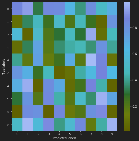
x = torch.rand(1, 10, 10)
lif = TestNode(threshold=0.3, tau=2.)
## Reset Before use
lif.n_reset()
spike = lif(x)
spike_rate_vis(x)

All neurons need to be reset before use to ensure that the membrane potential of the neuron is at resting potential. The above code allows the visualization of the input currents and pulses of the neuron.

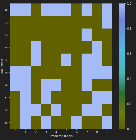
BrainCog also supports efficient simulation of neurons on a larger scale and allows easy visualization of the behavior of neurons in terms of spiking rate.

lif = TestNode(threshold=0.5)
x = torch.rand(100, 100)
spike = []

lif.n_reset()
for t in range(50):
spike.append(lif(x))

spike = torch.stack(spike)
spike_rate_vis(spike)

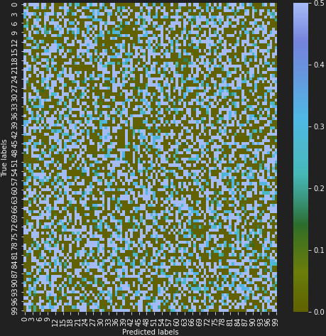
BrainCog also supports time-domain analysis of different neurons. The following code implements the time-domain behavior analysis of neurons.

lif = IzhNode(threshold=0.5, tau=2.)
x = torch.rand(100)
spike = []

lif.n_reset()
for t in range(1000):
spike.append(lif(50 * x))

spike = torch.stack(spike)

spike_rate_vis_1d(spike)

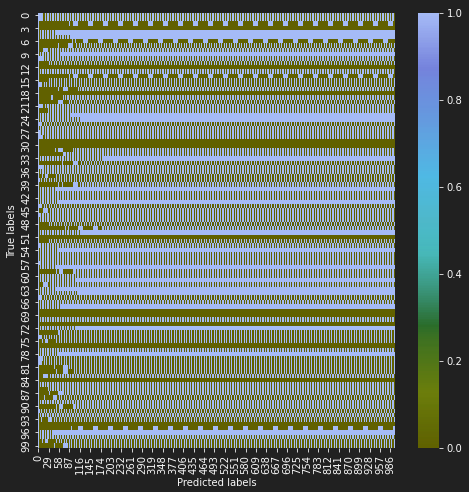
Of course, we can also use braincog to analyze the behavior of a neuron in detail.

spike_rate_vis_1d(spike)
#%%
lif = IzhNode(threshold=.5)
lif.n_reset()
lif.requires_fp = True

mem = []
spike = []
for t in range(100):
x = torch.tensor(10)
# x = torch.rand(1)
spike.append(lif(x))
mem.append(lif.mem)

mem = torch.stack(mem)
spike = torch.stack(spike)

outputs = torch.max(mem, spike).detach().cpu().numpy()

plt.plot(outputs)
plt.savefig('lif.pdf', bbox_inches='tight')

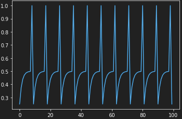
The figure above shows the behavior of a LIF neuron with a constant current input.

Braincog provides an easy-to-use interface for neuron construction, neuron simulation and visualization.