Lec 4 Building Efficient Spiking Neural Networks with BrainCog

Hello, in this tutorial, we will share with you how to build and train high performance spiking neural networks using BrainCog.

Creating neuron classes

Import the braincog package

from functools import partial
from timm.models import register_model
from braincog.base.node.node import *
from braincog.base.encoder.encoder import *
from braincog.model_zoo.base_module import BaseModule, BaseConvModule
from braincog.datasets import is_dvs_data
from braincog.datasets.datasets import get_dvsc10_data
from braincog.base.utils.visualization import spike_rate_vis, spike_rate_vis_1d

Defining a new neural network

Note that all SNNs need to inherit from BaseModule. BaseModule implements some basic interfaces for neuron state control and visualization in SNNs.

@register_model  ## register model in timm
class SNN5(BaseModule):
    def __init__(self,
                 num_classes=10,
                 step=8,
                 node_type=LIFNode,
                 encode_type='direct',
                 *args,
                 **kwargs):
        super().__init__(step, encode_type, *args, **kwargs)
        self.num_classes = num_classes

        self.node = node_type
        if issubclass(self.node, BaseNode):
            self.node = partial(self.node, **kwargs, step=step)

        self.dataset = kwargs['dataset'] if 'dataset' in kwargs else 'dvsc10'
        if not is_dvs_data(self.dataset):
            init_channel = 3
        else:
            init_channel = 2

        self.feature = nn.Sequential(
            BaseConvModule(init_channel, 16, kernel_size=(3, 3), padding=(1, 1), node=self.node),
            BaseConvModule(16, 64, kernel_size=(5, 5), padding=(2, 2), node=self.node),
            nn.AvgPool2d(2),
            BaseConvModule(64, 128, kernel_size=(5, 5), padding=(2, 2), node=self.node),
            nn.AvgPool2d(2),
            BaseConvModule(128, 256, kernel_size=(3, 3), padding=(1, 1), node=self.node),
            nn.AvgPool2d(2),
            BaseConvModule(256, 512, kernel_size=(3, 3), padding=(1, 1), node=self.node),
            nn.AvgPool2d(2),
        )
        self.fc = nn.Sequential(
            nn.Flatten(),
            nn.Linear(512 * 3 * 3, self.num_classes),
        )

    def forward(self, inputs):
        inputs = self.encoder(inputs)
        self.reset()

        if self.layer_by_layer:
            x = self.feature(inputs)
            x = self.fc(x)
            x = rearrange(x, '(t b) c -> t b c', t=self.step).mean(0)
            return x

        else:
            outputs = []
            for t in range(self.step):
                x = inputs[t]
                x = self.feature(x)
                x = self.fc(x)
                outputs.append(x)

            return sum(outputs) / len(outputs)

The BaseModule provides an easy-to-call interface for controlling the behavior of neurons in the network. For example, it is possible to reset the membrane potentials of all neurons in the network by simply calling self.reset(). Thus, it is only necessary to implement __init__() and forward() to build a spiking neural network using braincog.

Dataset initialization

BrainCog provides interfaces to several datasets including image datasets and event datasets. Examples include MNIST, CIFAR10, ImageNet, DVS-CIFAR10, DVS-Gesture, N-Caltech101.

When using datasets, the following code can be used to implement them:

train_loader, _, _, _ = get_dvsc10_data(batch_size=1, step=8)
it = iter(train_loader)
inputs, labels = it.next()
print(inputs.shape, labels.shape)
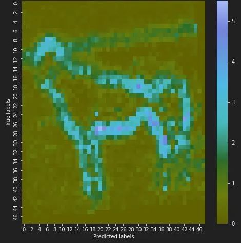
spike_rate_vis(inputs[0, :, 0])

Out[1]: torch.Size([1, 8, 2, 48, 48]) torch.Size([1])

Model Inference and Visualization

After defining the model and acquiring the dataset, the model can be used for forward inference.

model = SNN5(layer_by_layer=True, datasets='dvsc10').cuda()
print(model)

Out[2]: 
SNN5(
  (encoder): Encoder()
  (feature): Sequential(
    (0): BaseConvModule(
      (conv): Conv2d(2, 16, kernel_size=(3, 3), stride=(1, 1), padding=(1, 1), bias=False)
      (preact): Identity()
      (bn): BatchNorm2d(16, eps=1e-05, momentum=0.1, affine=True, track_running_stats=True)
      (node): LIFNode(
        (act_fun): QGateGrad()
      )
      (activation): Identity()
    )
    (1): BaseConvModule(
      (conv): Conv2d(16, 64, kernel_size=(5, 5), stride=(1, 1), padding=(2, 2), bias=False)
      (preact): Identity()
      (bn): BatchNorm2d(64, eps=1e-05, momentum=0.1, affine=True, track_running_stats=True)
      (node): LIFNode(
        (act_fun): QGateGrad()
      )
      (activation): Identity()
    )
    (2): AvgPool2d(kernel_size=2, stride=2, padding=0)
    (3): BaseConvModule(
      (conv): Conv2d(64, 128, kernel_size=(5, 5), stride=(1, 1), padding=(2, 2), bias=False)
      (preact): Identity()
      (bn): BatchNorm2d(128, eps=1e-05, momentum=0.1, affine=True, track_running_stats=True)
      (node): LIFNode(
        (act_fun): QGateGrad()
      )
      (activation): Identity()
    )
    (4): AvgPool2d(kernel_size=2, stride=2, padding=0)
    (5): BaseConvModule(
      (conv): Conv2d(128, 256, kernel_size=(3, 3), stride=(1, 1), padding=(1, 1), bias=False)
      (preact): Identity()
      (bn): BatchNorm2d(256, eps=1e-05, momentum=0.1, affine=True, track_running_stats=True)
      (node): LIFNode(
        (act_fun): QGateGrad()
      )
      (activation): Identity()
    )
    (6): AvgPool2d(kernel_size=2, stride=2, padding=0)
    (7): BaseConvModule(
      (conv): Conv2d(256, 512, kernel_size=(3, 3), stride=(1, 1), padding=(1, 1), bias=False)
      (preact): Identity()
      (bn): BatchNorm2d(512, eps=1e-05, momentum=0.1, affine=True, track_running_stats=True)
      (node): LIFNode(
        (act_fun): QGateGrad()
      )
      (activation): Identity()
    )
    (8): AvgPool2d(kernel_size=2, stride=2, padding=0)
  )
  (fc): Sequential(
    (0): Flatten(start_dim=1, end_dim=-1)
    (1): Linear(in_features=4608, out_features=10, bias=True)
  )
)

The above code shows the instantiation process of the SNN model, so that we get an instance of SNN5, and then we can use this instance for inference.

outputs = model(inputs.cuda())
print(outputs)

Out[3]: tensor([[-0.0524,  0.1208, -0.0167, -0.1197, -0.0659, -0.0528, -0.1191, -0.0732, -0.0615,  0.1520]], device='cuda:0', grad_fn=<MeanBackward1>)

The event data is fed into the model to get the output of the event data belonging to different categories. Since the model has not been trained, the output is random.

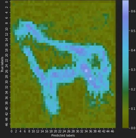
The BaseModule in braincog also provides visualization methods to easily capture the activity of each layer of neurons.

model.set_requires_fp(True)
outputs = model(inputs.cuda())
feature_map = model.get_fp()

feature = feature_map[0]
feature = rearrange(feature, '1 (t c) ... -> t c ...', t=8)
spike_rate_vis(feature[:, 0].detach())
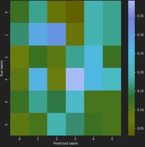
feature = feature_map[-1]

feature = rearrange(feature, '1 (t c) ... -> t c ...', t=8)
spike_rate_vis(feature[:, 0].detach())

The above section shares how to build spiking neural networks using braincog.

braincog also provides scripts for training high performance spiking networks.

It can be found at https://github.com/BrainCog-X/Brain-Cog/blob/main/examples/Perception_and_Learning/img_cls/bp/main.py.

Braincog also provides some model benchmarks for your reference when designing SNNs. The predefined models can be found at https://github.com/BrainCog-X/Brain-Cog/tree/main/braincog/model_zoo.

The benchmark results of the models can be found at https://github.com/BrainCog-X/Brain-Cog/tree/main/examples/Perception_and_Learning/img_cls/bp.